

![]()
Pythia tutorial setup
This is a web page for the Pythia event generator tutorials held at the MCnet school 2019 in Quy Nhon. The description borrows massively from the CTEQ 2019 tutorial setup and the MCnet London 2019 tutorial setup designed by S. Hoeche and S. Prestel. The instructions are based on the Pythia 8.2 Worksheet by Torbjörn Sjöstrand and Stefan Prestel.
Container option (preferred!)
This tutorial uses containers. Please install docker on your personal computer prior to the tutorial.
Installation instructions for docker can be found here. On Linux systems, create a
group "docker" and add yourself to it to avoid having to run all docker commands as sudo:
sudo groupadd docker
sudo usermod -aG docker $USER
If you have questions on installing docker or on testing the docker environment, please ask the lecturers
before the tutorial. Due to time constraints we cannot assist everyone with setting up docker during the tutorial itself.
Download
The docker container images can be pulled directly from dockerhub. The command line for this is
docker pull mcnetschool/tutorial:pythia-1.0.0
The docker image will then be downloaded to /var/lib/docker.
Alternatively, the container images can be downloaded from here.
These latter images must be loaded into docker
explicitly. The command line for this reads
docker load -i mcnetschool-tutorial-pythia-8.2.43.tar.bz2
The tutorial material is obtained from Bitbucket. You can clone the repository using
hg clone https://bitbucket.org/Patrick_K_2016/mcnet-tutorial-vietnam
The tutorial instructions are given below.
Running the containers
We recommend to run the containers for the MC tutorials in the mcnet-tutorial-vietnam directory and using your actual
user-id. In order to run Pythia,
execute the shell command
docker run -it -u $(id -u $USER) -v $PWD:$PWD -w $PWD --env="RIVET_ANALYSIS_PATH=." mcnetschool/tutorial:pythia-1.0.0
The option -v will mount your current working directory $PWD to a container directory
with the same name. This allows the container to access your local files and to write files
to the current working directory.
You may consider adding the --rm flag to automatically clean up after your
container exits. Note that in this case
all modifications you may have made to the container will be lost.
On Windows 10 laptops, you can start the docker run with
docker run -it -u 1000 -v %cd%:/home -w /home --env="RIVET_ANALYSIS_PATH=." mcnetschool/tutorial:pythia-1.0.0
The operating system will then ask you for permission to access the shared folder.
Running the tutorials
Instructions for the Pythia tutorials are given below. Please work in the mcnet-tutorial-vietnam/Pythia/ directory checked out from Bitbucket.
Virtual machine setup (deprecated, last resort)
In case of insurmountable problems with docker you may use a legacy virtual machine. In this case, please install Oracle Virtual Box on your personal computer prior to the tutorial. If you have questions on installing VirtualBox, please ask the lecturers before the tutorial. Due to time constraints we cannot assist everyone with setting up the environment during the tutorial itself.
Download
The virtual machine disk can be downloaded from here. Unarchive the disk using 7-Zip. If 7-Zip is missing on your Linux system, install the package p7zip. On Windows, download the 7-Zip executable from here. On MacOS, use the unarchiver.
Creating the Virtual Machine
Create a new machine with VirtualBox using the GUI. In the first step, VirtualBox will ask for the name of the machine and its OS. For the latter choose Linux -> Ubuntu (64 bit). In the next step, set the size of the memory. About 1GB should be fine. In the last step, select the virtual disk. Choose 'Use an existing virtual hard drive file' and open the *.vdi file you just downloaded and extracted.
Before starting the virtual machine, enter its settings and increase the video RAM size to at least 48MB (Settings -> Display -> Video). If you have more than two processor cores on your host system, allow the VM to use two cores (Settings -> System -> Processor). You must enable hardware virtualization in your BIOS to do this!
Starting the Virtual Machine
We are booting a lightweight Linux, which you can customize.
The login name is student, the password is 2019.
The keyboard layout can be set using the layout switcher in the task bar, or by running setxkbmap LC in the terminal, where LC is your
language code (us, de,...).
Common tools which are installed include xterm, lxterminal, vi, emacs, gv, evince and firefox. If you need root privileges to install further programs of your choice, use sudo. Note that the package information has been purged, and you need to run sudo aptitude update before any other command.
Running the tutorial
The virtual machine image that you've downloaded was originally designed for the CTEQ 2019 school tutorial (by S. Hoeche). Thus, the tutorial instructions shipped with this virtual machine do not apply for the MCnet school 2019.
The correct tutorial instructions are given below . First, create
a directory mcnet2019 as subdirectory in the home directory. Enter this new directory and
clone the repository using
hg clone https://bitbucket.org/Patrick_K_2016/mcnet-tutorial-vietnam.
Within mcnet-tutorial-vietnam, you will find the Pythia/ directory. For the Pythia tutorial, please refer to the material in this directory and the instructions below.
1 Introduction
The Pythia 8.2 program is a standard tool for the generation of high-energy collisions (specifically, it focuses on centre-of-mass energies greater than about 10 GeV), comprising a coherent set of physics models for the evolution from a few-body high-energy (“hard”) scattering process to a complex multihadronic final state. The particles are produced in vacuum. Simulation of the interaction of the produced particles with detector material is not included in Pythia but can, if needed, be done by interfacing to external detector-simulation codes.
The Pythia 8.2 code package contains a library of hard interactions and models for initial- and final-state parton showers, multiple parton-parton interactions, beam remnants, string fragmentation and particle decays. It also has a set of utilities and interfaces to external programs.
The objective of this exercise is to teach you the basics of how to use the Pythia 8.2 event generator to study various physics aspects. As you become more familiar you will better understand the tools at your disposal, and can develop your own style to use them. Within this first exercise it is not possible to describe the physics models used in the program; for this we refer to the Pythia 8.2 introduction [1], to the full Pythia 6.4 physics description [2], and to all the further references found in them.
Pythia 8 is, by today’s standards, a small package. It is completely self-contained, and is therefore easy to install for standalone usage, e.g. if you want to have it on your own laptop, or if you want to explore physics or debug code without any danger of destructive interference between different libraries. Section 2 describes the installation procedure, which is what we will need for this introductory session. It does presuppose a working Unix-style environment with C++ compilers and the like; check Appendix D if in doubt.
When you use Pythia you are expected to write the main program yourself, for maximal flexibility and power. Several examples of such main programs are included with the code, to illustrate common tasks and help getting started. Section 3 gives you a simple step-by-step recipe how to write a minimal main program, that can then gradually be expanded in different directions, e.g. as in Section 4.
In Section 5 you will see how the parameters of a run can be read in from a file, so that the main program can be kept fixed. Many of the provided main programs therefore allow you to create executables that can be used for different physics studies without recompilation, but potentially at the cost of some flexibility.
Note for the MCnet school tutorial 2019: You should view this tutorial sheet also as a user reference. So do not be scared of the length of the document. For a one-day tutorial session, you should be able to complete Section 6 on parton shower uncertainties in top pair production. Section 7 then gives you the opportunity to explore some topics beyond the scope of the MCnet tutorial.
While Pythia can be run standalone, it can also be interfaced with a set of other libraries. One example is HepMC, which is the standard format used by experimentalists to store generated events. Since the HepMC library location is installation-dependent it is not possible to give a fool-proof linking procedure, but some hints are provided for the interested in Appendix C. Further main programs included with the Pythia code provide examples of linking, e.g., to AlpGen, MadGraph, PowHeg, FastJet, Root, and the Les Houches Accords LHEF, LHAPDF and SLHA.
Appendix A contains a brief summary of the event-record structure, and Appendix B some notes on simple histogramming and jet finding. Appendices C and D have already been mentioned.
2 Installation
Note for the MCnet school tutorial 2019: You find the Pythia Docker image and instructions above. After you pulled the docker container (or downloaded the virtual machine), do make sure that your working directory contains the latest version of the tutorial files from the bitbucket repository. We will refer to the directory mcnet-tutorial-vietnam/Pythia as examples directory below. Further examples can be found in /usr/local/share/Pythia8/examples/ within the docker container. Your image already contains a very general installation of Pythia 8 (version 8.243). Thus, you do not need to follow the installation instructions, and may directly continue with section 3. The following instructions here are kept for reference, in case you want to install Pythia 8 on your private machine (which should not be too hard).
Denoting a generic Pythia 8 version pythia82xx (at the time of writing xx = 43), here is how to install Pythia 8 on a Linux/Unix/MacOSX system as a standalone package (assuming you have standard Unix-family tools installed, see Appendix D).
- In a browser, go to
http://home.thep.lu.se/Pythia - Download the (current) program package
pythia82xx.tgz
to a directory of your choice (e.g. by right-clicking on the link). - In a terminal window, cd to where pythia82xx.tgz was downloaded, and type
tar xvfz pythia82xx.tgz
This will create a new (sub)directory pythia82xx where all the Pythia source files are now ready and unpacked. - Move to this directory (cd pythia82xx) and do a make. This will take ~3 minutes (computer-dependent). The Pythia 8 library is now compiled and ready for physics.
- For test runs, cd to the examples/ subdirectory. An ls reveals a list of programs,
mainNN.cc, with NN from 01 through 28 (and beyond). These example programs
each illustrate an aspect of Pythia 8. For a list of what they do, see the “Sample
Main Programs” page in the online manual (point 6 below).
Initially only use one or two of them to check that the installation works. Once you have worked your way though the introductory exercises in the next sections you can return and study the programs and their output in more detail.
To execute one of the test programs, do
make mainNN
./mainNN
The output is now just written to the terminal, stdout. To save the output to a file instead, do ./mainNN > outNN, after which you can study the test output at leisure by opening outNN. See Appendix A for an explanation of the event record that is listed in several of the runs. - If you use a web browser to open the file
pythia82xx/share/Pythia8/htmldoc/Welcome.html
you will gain access to the online manual, where all available methods and parameters are described. Use the left-column index to navigate among the topics, which are then displayed in the larger right-hand field.
3 A “Hello World” program
We will now generate a single gg → tt event at the LHC, using Pythia standalone.
Open a new file mymain01.cc in the examples subdirectory with a text editor, e.g. Emacs. Then type the following lines (here with explanatory comments added):
#include "Pythia8/Pythia.h" // Include Pythia headers.
using namespace Pythia8; // Let Pythia8:: be implicit.
int main() { // Begin main program.
// Set up generation.
Pythia pythia; // Declare Pythia object
pythia.readString("Top:gg2ttbar = on"); // Switch on process.
pythia.readString("Beams:eCM = 8000."); // 8 TeV CM energy.
pythia.init(); // Initialize; incoming pp beams is default.
// Generate event(s).
pythia.next(); // Generate an(other) event. Fill event record.
return 0;
} // End main program with error-free return.
The examples/Makefile has been set up to compile all mymainNN.cc, NN = 01 - 99, and link
them to the lib/libpythia8.a library, just like the mainNN.cc ones. Therefore you can
compile and run mymain01 as before:
make mymain01
./mymain01 > myout01
If you want to pick another name, or if you need to link to more libraries, you have to edit
examples/Makefile appropriately.
Thereafter you can study myout01, especially the example of a complete event record (preceded by initialization information, and by kinematical-variable and hard-process listing for the same event). At this point you need to turn to Appendix A for a brief overview of the information stored in the event record.
An important part of the event record is that many copies of the same particle may exist, but only those with a positive status code are still present in the final state. To exemplify, consider a top quark produced in the hard interaction, initially with positive status code. When later a shower branching t → tg occurs, the new t and g are added at the bottom of the then-current event record, but the old t is not removed. It is marked as decayed, however, by negating its status code. At any stage of the shower there is thus only one “current” copy of the top. After the shower, when the final top decays, t → bW+, also that copy receives a negative status code. When you understand the basic principles, see if you can find several copies of the top quarks, and check the status codes to figure out why each new copy has been added. Also note how the mother/daughter indices tie together the various copies.
4 A first realistic analysis
We will now gradually expand the skeleton mymain01 program from above, towards what would be needed for a more realistic analysis setup.
- Often, we wish to mix several processes together. To add the process qq → tt to the
above example, just include a second pythia.readString call
pythia.readString("Top:qqbar2ttbar = on"); - Now we wish to generate more than one event. To do this, introduce a loop around
pythia.next(), so the code now reads
for (int iEvent = 0; iEvent < 5; ++iEvent) {
pythia.next();
}
Hereafter, we will call this the event loop. The program will now generate 5 events; each call to pythia.next() resets the event record and fills it with a new event. To list more of the events, you also need to add
pythia.readString("Next:numberShowEvent = 5");
along with the other pythia.readString commands. - To obtain statistics on the number of events generated of the different kinds, and
the estimated cross sections, add a
pythia.stat();
just before the end of the program. - During the run you may receive problem messages. These come in three kinds:
- a warning is a minor problem that is automatically fixed by the program, at least approximately;
- an error is a bigger problem, that is normally still automatically fixed by the program, by backing up and trying again;
- an abort is such a major problem that the current event could not be completed; in such a rare case pythia.next() is false and the event should be skipped.
Thus the user need only be on the lookout for aborts. During event generation, a problem message is printed only the first time it occurs (except for a few special cases). The above-mentioned pythia.stat() will then tell you how many times each problem was encountered over the entire run.
- Studying the event listing for a few events at the beginning of each run is useful to make
sure you are generating the right kind of events, at the right energies, etc. For real
analyses, however, you need automated access to the event record. The Pythia event
record provides many utilities to make this as simple and efficient as possible. To access
all the particles in the event record, insert the following loop after pythia.next() (but
fully enclosed by the event loop)
for (int i = 0; i < pythia.event.size(); ++i) {
cout << "i = " << i << ", id = "
<< pythia.event[i].id() << endl;
}
which we will call the particle loop. Inside this loop, you can access the properties of each particle pythia.event[i]. For instance, the method id() returns the PDG identity code of a particle (see Appendix A.1). The cout statement, therefore, will give a list of the PDG code of every particle in the event record. - As mentioned above, the event listing contains all partons and particles, traced
through a number of intermediate steps. Eventually, the top will decay (t → Wb),
and by implication it is the last top copy in the event record that defines the
definitive top production kinematics, just before the decay. You can obtain the
location of this final top e.g. by inserting a line just before the particle loop
int iTop = 0;
and a line inside the particle loop
if (pythia.event[i].id() == 6) iTop = i;
The value of iTop will be set every time a top is found in the event record. When the particle loop is complete, iTop will now point to the final top in the event record (which can be accessed as pythia.event[iTop]). - In addition to the particle properties in the event listing, there are also methods that return many derived quantities for a particle, such as transverse momentum, pythia.event[iTop].pT(), and pseudorapidity, pythia.event[iTop].eta(). Use these methods to print out the values for the final top found above.
- We now want to generate more events, say 1000, to view the shape of these distributions.
Inside Pythia is a very simple histogramming class, see Appendix B.1, that can be used
for rapid check/debug purposes. To book the histograms, insert before the event loop
Hist pT("top transverse momentum", 100, 0., 200.);
Hist eta("top pseudorapidity", 100, -5., 5.);
where the last three arguments are the number of bins, the lower edge and the upper edge of the histogram, respectively. Now we want to fill the histograms in each event, so before the end of the event loop insert
pT.fill( pythia.event[iTop].pT() );
eta.fill( pythia.event[iTop].eta() );
Finally, to write out the histograms, after the event loop we need a line like
cout << pT << eta;
Do you understand why the η distribution looks the way it does? Propose and study a related but alternative measure and compare. - As a final standalone exercise, consider plotting the charged multiplicity of events. You then need to have a counter set to zero for each new event. Inside the particle loop this counter should be incremented whenever the particle isCharged() and isFinal(). For the histogram, note that it can be treacherous to have bin limits at integers, where roundoff errors decide whichever way they go. In this particular case only even numbers are possible, so 100 bins from -1 to 399 would still be acceptable.
5 Input files
With the mymain01.cc structure developed above it is necessary to recompile the main program for each minor change, e.g. if you want to rerun with more statistics. This is not time-consuming for a simple standalone run, but may become so for more realistic applications. Therefore, parameters can be put in special input “card” files that are read by the main program.
We will now create such a file, with the same settings used in the mymain01.cc example program. Open a new file, mymain01.cmnd, and input the following
Beams:idA = 2212 ! first incoming beam is a 2212, i.e. a proton.
Beams:idB = 2212 ! second beam is also a proton.
Beams:eCM = 8000. ! the cm energy of collisions.
Top:gg2ttbar = on ! switch on the process g g -> t tbar.
Top:qqbar2ttbar = on ! switch on the process q qbar -> t tbar.
The mymain01.cmnd file can contain one command per line, of the type
variable = value
All variable names are case-insensitive (the mixing of cases has been chosen purely to improve
readability) and non-alphanumeric characters (such as !, # or $) will be interpreted as the
start of a comment. All valid variables are listed in the online manual (see Section
2, point 6, above). Cut-and-paste of variable names can be used to avoid spelling
mistakes.
The final step is to modify our program to use this input file. The name of this input
file can be hardcoded in the main program, but for more flexibility, it can also be
provided as a command-line argument. To do this, replace the int main() { line by
int main(int argc, char* argv[]) {
and replace all pythia.readString(...) commands with the single command
pythia.readFile(argv[1]);
The executable mymain01 is then run with a command line like
./mymain01 mymain01.cmnd > myout01
and should give the same output as before.
In addition to all the internal Pythia variables there exist a few defined in the database but not
actually used. These are intended to be useful in the main program, and thus begin with
Main:. The most basic of those is Main:numberOfEvents, which you can use to specify
how many events you want to generate. To make this have any effect, you need to
read it in the main program, after the pythia.readFile(...) command, by a line
like
int nEvent = pythia.mode("Main:numberOfEvents");
and set up the event loop like
for (int iEvent = 0; iEvent < nEvent; ++iEvent) {
You are now free to play with further options in the input file, such as:
- PartonLevel:FSR = off
switch off final-state radiation. - PartonLevel:ISR = off
switch off initial-state radiation. - PartonLevel:MPI = off
switch off multiparton interactions. - Tune:pp = 3 (or other values between 1 and 17)
different combined tunes, in particular to radiation and multiparton interactions parameters. In part this reflects that no generator is perfect, and also not all data is perfect, so different emphasis will result in different optima. - Random:setSeed = on
Random:seed = 123456789
all runs by default use the same random-number sequence, for reproducibility, but you can pick any number between 1 and 900,000,000 to obtain a unique sequence.
For instance, check the importance of FSR, ISR and MPI on the charged multiplicity of events by switching off one component at a time.
The possibility to use command-line input files is further illustrated e.g. in main16.cc and main42.cc.
The online manual also exists in an interactive variant, where you semi-automatically can construct a file with all the command lines you wish to have. This requires that somebody installs the pythia82xx/share/Pythia8/phpdoc directory in a webserver. This is not a commercial-quality product, however, and requires some user discipline. Full instructions are provided on the “Save Settings” page.
You have now completed the core part of the worksheet — congratulations! The next section is devoted to shower uncertainties. The section after that will then allow you to take off in different directions, depending on your interests, and if you are still hungry for more.
6 Shower uncertainties in top pair production
Event generators try to implement the most precise and complete description of scattering events. The simulation will contain uncertainties because a) the calculation of some mechanism might been approximated (e.g. by calculating only to a certain perturbative order), or b) if a first-principles calculation of a particular phenomenon is not yet known. Uncertainties due to b) are very difficult to quantify without dedicated studies. In the following, we will consider uncertainties of the type a) that stem from truncating perturbation theory at some order. Such variations have been considered in [13] and are documented under the menu item “Automated Shower Variations” in the Pythia online manual.
Parton showers are a crucial component in a realistic event simulation. They are approximations to perturbative all-order QCD, which model the structure and evolution of jets of partons. In this section, we will investigate some of the uncertainties of a parton shower calculation.
Note for the MCnet school tutorial 2019: We will use the Rivet analysis tool for this, so that you can easily compare your results to predictions from other generators. Rivet relies on HepMC event input. Thus, you can follow the instructions in App. C to upgrade your mymain.cc program to produce HepMC events. Alternatively, you can have a look at main41.cc and main42.cc in your examples directory. To avoid unnecessary delays, we recommend that you use the example main program mymain-hepmc.cc and the input file mymain-hepmc.cmnd that are provided in the bitbucket repository. This main program produces one HepMC file for each weight due to from shower variations. To avoid writing many events to disk, it is beneficial to declare the HepMC output files as FIFO pipes. Your system will then flush the output files after Rivet has read and analysed the events, thus ensuring that no large files have to be stored. We provide the bash script run.sh to handle this task. Have a look at mymain-hepmc.cc and run.sh to make sure you understand what is going on before proceeding!
Parton showers resum large logarithmic enhancements by using (QCD) perturbation theory. They contain a dependence on renormalisation/factorisation scales, and on non-logarithmic pieces that are contained in the splitting functions that are used to define the shower. Pythia allows you [13] to vary
- The renormalization scale in final-state and initial-state splittings;
- The finite pieces of the splitting functions used for final-state and initial-state splittings.
We will use both of these to assess which piece of the perturbative calculation produces significant uncertainties for particular observables. Please note that these variations do not span the real envelope of all event generator uncertainties. However, getting a feeling for the perturbative uncertainties is still a useful skill.
6.1 Shower variations: Scales
To enable shower variations, you should first include the setting
UncertaintyBands:doVariations = on
in your input file mymain-hepmc.cmnd.
Let us first look varying the renormalization scale in the parton shower, and consider variations in final-state and initial-state splittings separately. For this, use the settings
scale_fsr_lo fsr:muRfac=0.5,
scale_fsr_hi fsr:muRfac=2.0,
scale_isr_lo isr:muRfac=0.5,
scale_isr_hi isr:muRfac=2.0
}
The labels scale_fsr_lo etc. are arbitrary, and have no influence on the result. The first line
means that Pythia will produce an additional event weight that contains the result of
evaluating all final-state splittings with αs( μrPS), and similarly for the following three
lines. Thus, Pythia will produce four additional event weights that can be used for
histogramming. Before moving forward, check if the variation of these weights are
reasonable.
μrPS), and similarly for the following three
lines. Thus, Pythia will produce four additional event weights that can be used for
histogramming. Before moving forward, check if the variation of these weights are
reasonable.
Instructions for the MCnet school tutorial 2019: Use the script run.sh provided in the bitbucket repository. In this way, you will be able to produce uncertainty envelopes relatively conveniently. In order to produce the results for this section, update the input file mymain-hepmc.cmnd with the uncertainty settings listed above and run
in the tutorial directory. This will produce files that contain the results for each variation (scale_fsr_lo.yoda, scale_fsr_hi.yoda, scale_isr_lo.yoda, scale_isr_hi.yoda), and three files that contain the envelope of final-state shower variations (pythiaScalesFSR.yoda), of initial-state shower variations (pythiaScalesISR.yoda) and a combined envelope (pythiaScales.yoda). Plots will be stored in a directory called pythiaScales. Check that the weight variation is reasonable by including output in mymain-hepmc.cc (and recompiling). If this is not the case, try to understand why. It is also possible to produce the variations separately by running four times using the different settings
- SpaceShower:renormMultFac = 0.5 (equivalent to scale_isr_lo)
- SpaceShower:renormMultFac = 2.0 (equivalent toscale_isr_hi)
- TimeShower:renormMultFac = 0.5 (equivalent to scale_fsr_lo)
- TimeShower:renormMultFac = 2.0 (equivalent to scale_fsr_hi)
What are the benefits and downsides of performing separate runs? Note that separate runs might turn out to be the preferred option for scale variations of the showers.
Now examine your histograms and try to answer
- For which observable do you find the largest final-state shower variation? Why?
- For which observable do you find the largest initial-state shower variation? Why?
- Do the variation bands have features? Can you explain the features?
6.2 Shower variations: Finite pieces
As a next step, let us check the impact of varying finite pieces of the splitting functions. For this, use
finitePieces_fsr_lo fsr:cNS=-2.0,
finitePieces_fsr_hi fsr:cNS=2.0,
finitePieces_isr_lo isr:cNS=-2.0,
finitePieces_isr_hi isr:cNS=2.0
}
Again, you will receive four additional weights that you can use for histogramming. You can check [13] on how these variations are defined. The variation of finite pieces in the splitting functions should not affect soft and collinear configurations too much.
Instructions for the MCnet school tutorial 2019: Use the script run.sh provided in the bitbucket repository. In order to produce the results for this section, update the input file mymain-hepmc.cmnd with the uncertainty settings listed above and run
in the tutorial directory. This will produce files that contain the results for each variation (finitePieces_fsr_lo.yoda, finitePieces_fsr_hi.yoda, finitePieces_isr_lo.yoda and finitePieces_isr_hi.yoda) and three files that contain the envelope of final-state shower variations (pythiaFinitesFSR.yoda), of initial-state shower variations (pythiaFinitesISR.yoda) and a combined envelope (pythiaFinites.yoda). Plots will be stored in a directory called pythiaFinites.
Examine your histograms and try to understand
- For which observable or in which phase space region do you find the largest effect?
- Can you find phase space regions in which this uncertainty dominates over the scale variations?
- What happens if you switch on/off matrix element corrections by invoking the settings TimeShower:MEcorrections and SpaceShower:MEcorrections?
This concludes the main part of the variations tutorial.
6.3 Shower variations: Bonus questions
If you still have time and you are willing to generate a large number of events, it might be interesting to check how your uncertainty estimate changes if you assume different correlations between the variations. For now, we have treated the variations as independent. If you e.g. use the settings
scale_shower_lo fsr:muRfac=0.5 isr:muRfac=0.5,
scale_shower_hi fsr:muRfac=2.0 isr:muRfac=2.0
}
instead, then Pythia will provide only two additional weights. The first of these weight is a combination of “down” variations, while the second gives a combination “up” variations. How does the envelope of these weights differ from your previous results? Would you expect significant differences?
7 Further studies
If you have time left, you should take the opportunity to try a few other processes or options. Below are given some examples, but feel free to pick something else that you would be more interested in.
- One popular misconception is that the energy and momentum of a B meson has to
be smaller than that of its mother b quark, and similarly for charm. The fallacy
is twofold. Firstly, if the b quark is surrounded by nearby colour-connected gluons,
the B meson may also pick up some of the momentum of these gluons. Secondly,
the concept of smaller momentum is not Lorentz-frame-independent: if the other
end of the b colour force field is a parton with a higher momentum (such as a beam
remnant) the “drag” of the hadronization process may imply an acceleration in the
lab frame (but a deceleration in the beam rest frame).
To study this, simulate b production, e.g. the process HardQCD:gg2bbbar. Identify B∕B* mesons that come directly from the hadronization, for simplicity those with status code -83 or -84. In the former case the mother b quark is in the mother1() position, in the latter in mother2() (study a few event listings to see how it works). Plot the ratio of B to b energy to see what it looks like. - One of the characteristics of multiparton-interactions (MPI) models is that they lead
to strong long-range correlations, as observed in data. That is, if many hadrons are
produced in one rapidity range of an event, then most likely this is an event where
many MPI’s occurred (and the impact parameter between the two colliding protons
was small), and then one may expect a larger activity also at other rapidities.
To study this, select two symmetrically located, one unit wide bins in rapidity (or pseudorapidity), with a variable central separation Δy:![[Δy ∕2, Δy ∕2 + 1]](worksheet-pythia8243-vietnam1x.png) and
and
![[- Δy ∕2 - 1,- Δy ∕2]](worksheet-pythia8243-vietnam2x.png) . For each event you may find nF and nB, the charged
multiplicity in the “forward” and “backward” rapidity bins. Suitable averages over
a sample of events then gives the forward–backward correlation coefficient
. For each event you may find nF and nB, the charged
multiplicity in the “forward” and “backward” rapidity bins. Suitable averages over
a sample of events then gives the forward–backward correlation coefficient
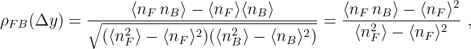
where the last equality holds for symmetric distributions such as in pp and pp.
Compare how ρFB(Δy) changes for increasing Δy = 0, 1, 2, 3,…, with and without MPI switched on (PartonLevel:MPI = on/off) for minimum-bias events (SoftQCD:nonDiffractive = on). - Z0 production to lowest order only involves one process, which is accessible with WeakSingleBoson:ffbar2gmZ = on. The problem here is that the process is ff → γ*∕Z0 with full γ*∕Z0 interference and so a significant enhancement at low masses. The combined particle is always classified with code 23, however. So generate events and study the γ*∕Z0 mass and p ⊥ distributions. Then restrict to a more “Z0-like” mass range with PhaseSpace:mHatMin = 75. and PhaseSpace:mHatMax = 120.
- Use a jet clustering algorithm, e.g. one of the SlowJet options described in Appendix B.2, to study the number of jets found in association with the Z0 above. You can switch off Z0 decay with 23:mayDecay = no, and negate its status code by pythia.event[iZ].statusNeg(), so that it will not be included in the jet finding. Here iZ is the last copy of the Z0, cf. how the last top copy was found above. Again check the importance of FSR/ISR/MPI.
Note that the Pythia homepage contains two further tutorials, in addition to older editions of the current one. We would like to mention one area of intense developments for event generators: Matching & merging the parton shower with multi-jet fixed-order matrix elements. Below, we give an introduction to the CKKW-L merging scheme implemented in Pythia.
7.1 CKKW-L merging
The main programs we have constructed and studied in the previous sections have one common drawback: all start from the Pythia 8 internal library of lowest-order processes, and then add higher-order corrections entirely by the internal parton-shower machinery. This will give reliable results for soft and collinear configurations, but less so for multiple hard, well-separated jets. To model the latter similarly well we need to include external input from higher-order calculations, at least at tree level, but where feasible also at one-loop level. A number of different external programs can provide such input, using the LHA/LHEF standard format [3, 4, 5] to transfer information, usually as LHE files. The hard-process events stored in these files will be accepted or rejected in such a way that doublecounting between different parton multiplicities is removed, resulting in a smooth transition between the multiplicities, and between the external input and the internal handling of parton showers. These two tasks usually go hand in hand.
Many different schemes have been proposed for matrix element + parton shower merging (MEPS), and a comprehensive selection of such schemes is available with the Pythia 8 distribution, including
- tree-level merging: MLM jet matching [6] (MadGraph- or AlpGen-style), CKKW-L merging [7], and unitarised ME+PS merging (UMEPS) [8]; and
- next-to-leading order merging: NL3 merging and unitarised NLO+PS merging (UNLOPS) [9].
The setup of such merging schemes is documented in the online manual, heading “Link to Other Programs”, page “Matching and Merging” with further subpages, and is illustrated in several of the example main programs.
Here we will experiment with the CKKW-L scheme, which was the first merging
scheme available in Pythia 8, and also is among the simpler to work with.
We will take the main80 example main program as a starting point for our
studies1 .
In its general structure it closely resembles the main program(s) we already constructed step by
step, so we will only need to comment on aspects that are new for the merging game. The
process W++ ≤ 2 jets will be taken as an example. It uses the LHE files
w+_production_lhc_0.lhe for W+ + 0 partons
w+_production_lhc_1.lhe for W+ + 1 parton
w+_production_lhc_2.lhe for W+ + 2 partons
in the examples directory to produce a result that simultaneously describes W+ + 0, 1, 2 jet
observables with leading-order matrix elements, while also including arbitrarily many shower
emissions. Jets are here defined by a clustering procedure on the partons thus generated. (We
omit other effects from consideration, such as MPIs or hadronization.)
Say we want to study a one-jet observable, e.g. the transverse momentum of the jet j in events
with exactly one jet. In this case, we want to take “hard” jets from the pp → Wj matrix
element (ME), while “soft” jets should be modelled by parton-shower (PS) emissions off the
pp → W states. In order to smoothly merge these two samples, we have to know in which
measure “hard” is defined, and which value of this measure separates the hard and soft regions.
In main80.cmnd, these definitions are
Merging:doKTMerging = on
Merging:ktType = 2
Merging:TMS = 30.
This will enable the merging procedure, with the merging scale defined by the minimal
longitudinally invariant k⊥ separation between partons (there are many other possibilities, by
ktType value or by your own choice of merging procedure), with a merging scale tMS = 30 GeV.
Such a definition fixes what we mean when we talk about “hard” and “soft” jets:
| Hard jets: | min{any relative k⊥ between sets of partons} > tMS |
| Soft jets: | min{any relative k⊥ between sets of partons} < tMS |
Thus, in order for the merging prescription to work, we need to remove phase space regions with min{any k⊥} < tMS from the W+1-parton matrix element calculation. Otherwise, there would be an overlap between the “soft jet” and “hard jet” samples.
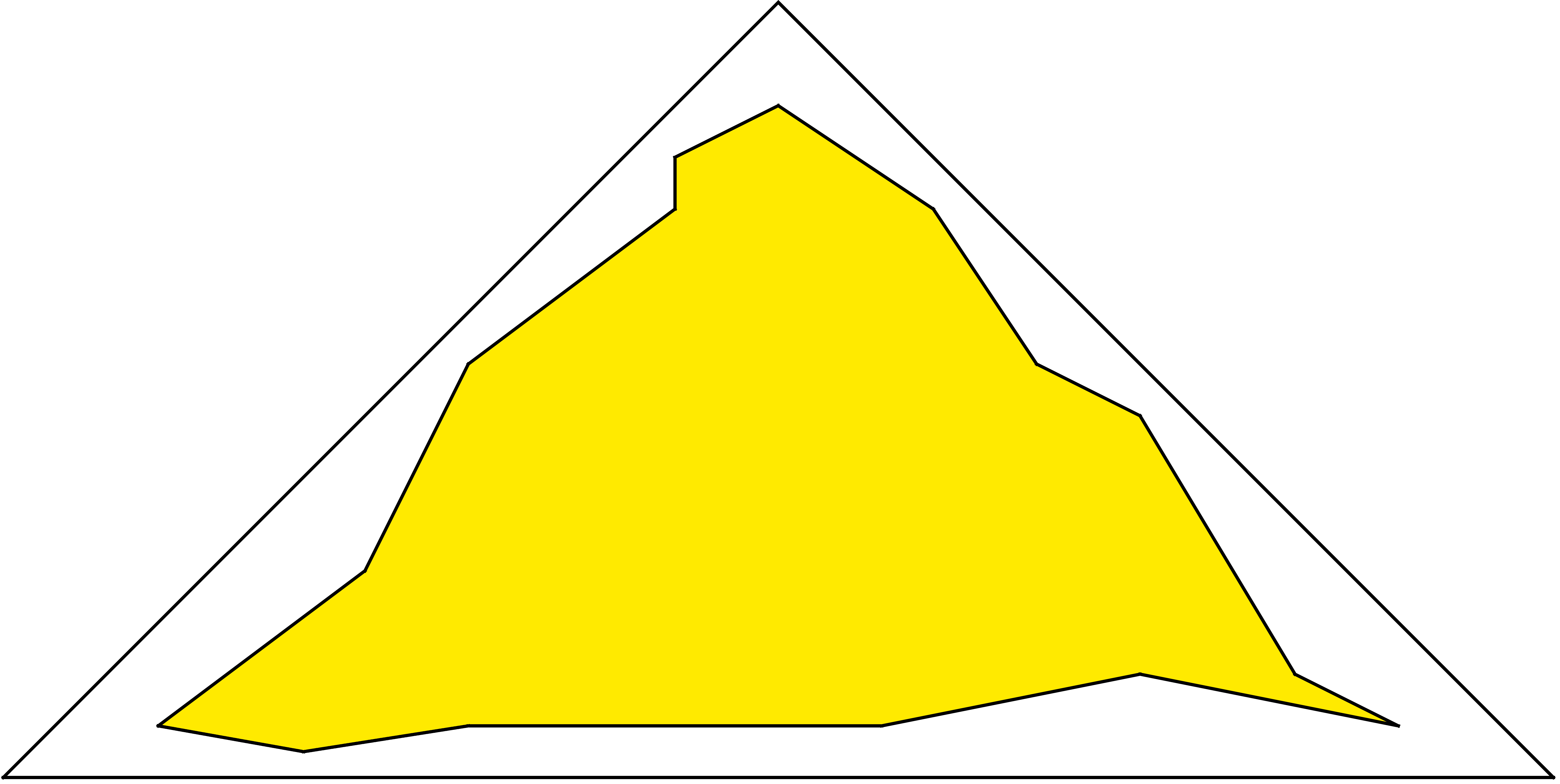
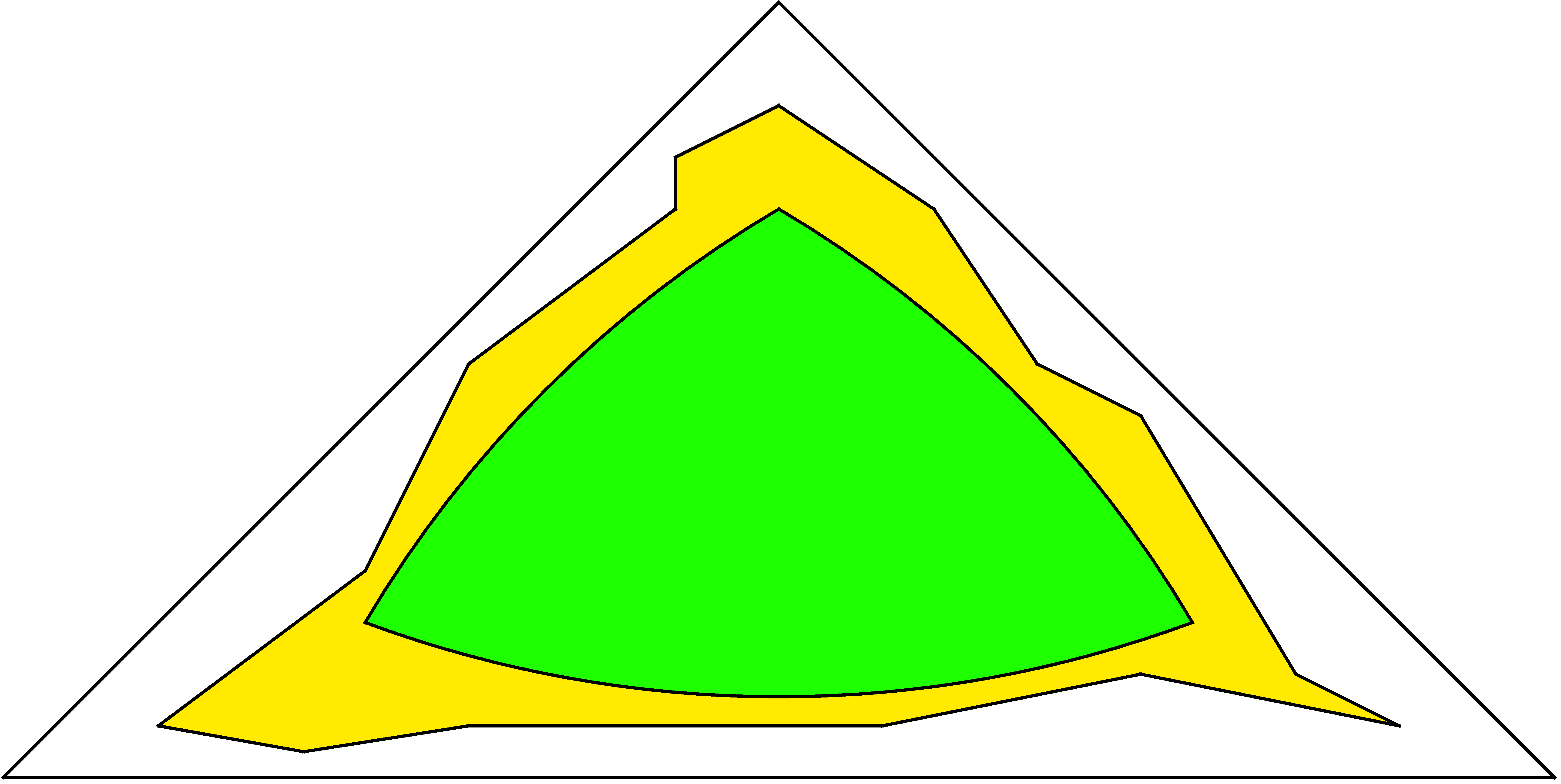
This requirement means that the merging-scale definition should be implemented as a cut in the matrix element generator. Alternatively, it is possible to enforce the cut in Pythia 8 internally, assuming that the ME is calculated with more inclusive (i.e. loose) cuts. This is illustrated in Figure 1, in which the triangle depicts the whole phase space, with soft or collinear divergences located on the edges. The yellow area symbolises the phase-space region used for the generation of the LHEF events, while the green area represents the phase space after Pythia 8 has enforced the merging-scale cut on the input events. In order to correctly apply the merging-scale cut, the green area has to be fully contained inside the yellow one, i.e. the cut in the ME generator has to be more inclusive than the tMS-cut. For optimal efficiency, the yellow and green areas should be identical. This can be the case in MadGraph 5 [10], when using the generation cuts ktdurham (corresponding to Merging:doKTMerging = on) and ptpythia (corresponding to Merging:doPTLundMerging = on).
After the merging-scale definition, we define the underlying process. To tell Pythia 8 that we
want to merge additional jets in W-boson production, we specify which is the core process,
using MadGraph notation, where the final state is defined by the W+ decay products rather
than by the W+ itself:
Merging:Process = pp>e+ve
in main80.cmnd. Finally, the setting
Merging:nJetMax = 2
tells the program to include the pre-generated ME events for up to two additional
jets.
In main80.cc, the input file main80.cmnd is read early on by the pythia.readFile(…)
command. This gives access to the number of events to be read from each LHE file, and the
number of LHE files to be processed. The subrun loop then handles each LHE file, one at a
time. Specifically, the
pythia.readFile("main80.cmnd", iMerge);
uses the iMerge argument when reading the main80.cmnd file, so that only those
commands following the respective Main:subrun = iMerge label are read. (Plus that
everything before the first Main:subrun is re-read, but that does not matter since
it stays the same.) Thus the proper LHE file is picked up for each jet multiplicity.
The
Beams:frameType = 4
also informs Pythia that beam parameters should be read from the header section of the LHE
file, and not set by the user.
Then we enter the event loop. The already-discussed difference in phase-space coverage can lead
to a fair fraction of all input events being rejected. Thus the number of produced events can be
lower than the requested Main:numberOfEvents one if the file is not large enough. (When no
further events can be read the pythia.next() command will return false, so that the event
loop can be exited at the end of the LHE file.) Those events that survive come with a
weight
double weight = pythia.info.mergingWeight();
which contains Sudakov factors (to remove the double counting between samples
of different multiplicity), αs ratios (to incorporate the αs running not available in
matrix element generators), and ratios of parton distributions (to include variable
factorization scales). This weight must be used when filling histogram bins, as is e.g. done
by
pTWnow.fill( pTW, weight);
for the p⊥ of the W boson. The sum of weights also goes into the calculation of the total
generated cross section.
After the event loop, the contribution to the p⊥ of the W boson from this particular multiplicity
is normalised by
pTWnow *= 1e9*pythia.info.sigmaGen()/(2.*pythia.info.nAccepted());
where the ratio of the two pythia.info numbers is the weight per event, the 1e9 is
for conversion from mb to pb, and the 2. compensates for the bin width to give
cross section per GeV. This number and more detailed statistics are printed to the
terminal. As a final step, the contribution of the current subrun is added to the total
histogram
pTWsum += pTWnow;
and the subrun loop begins over with the next LHE file. The complete histogram, combining all
multiplicities, is printed after the sub-run loop has concluded.
You can compile and run main80.cc by issuing the commands
make main80
./main80
When you run the program, note that some warning messages are issued routinely as part of the
merging machinery, in the steps where a clustering history is found and where it is decided
whether an event fails the merging scale cuts. Warnings from the SLHA interface also are
irrelevant. So no reason to worry about any of that.
After the first run with the main program as is, you can try different variations.
- Convince yourself that the variation of the “merging weight” is moderate.
- Check in which p⊥ regions which jet multiplicity contributes most.
- Study how the individual contributions and the sum changes when you run with a maximum of 1 or 0 jets, instead of the default 2.
- Compare the p⊥ spectrum of the W with what you get from running the internal Pythia production process, by straightforward modifications of your mymain01 program.
- Check the variation of merged predictions with tMS. You can do this by using an “inclusive” event sample, and having Pythia enforce a stronger tMS cut. In which phase-space region is the tMS variation most visible? A major limitation is the size of the event files that come with the standard Pythia distribution, for space reasons. If you have a decent Internet connection you can download larger files, with 100 000 events for each multiplicity up to W + 4 partons. Do this from the Pythia home page, in the “Tutorials” section of it, files wp_tree_0.lhe.gz through wp_tree_4.lhe.gz.
A The Event Record
The event record is set up to store every step in the evolution from an initial low-multiplicity partonic process to a final high-multiplicity hadronic state, in the order that new particles are generated. The record is a vector of particles, that expands to fit the needs of the current event (plus some additional pieces of information not discussed here). Thus event[i] is the i’th particle of the current event, and you may study its properties by using various event[i].method() possibilities.
The event.list() listing provides the main properties of each particles, by column:
- no, the index number of the particle (i above);
- id, the PDG particle identity code (method id());
- name, a plaintext rendering of the particle name (method name()), within brackets for initial or intermediate particles and without for final-state ones;
- status, the reason why a new particle was added to the event record (method status());
- mothers and daughters, documentation on the event history (methods mother1(), mother2(), daughter1() and daughter2());
- colours, the colour flow of the process (methods col() and acol());
- p_x, p_y, p_z and e, the components of the momentum four-vector (px,py,pz,E), in units of GeV with c = 1 (methods px(), py(), pz() and e());
- m, the mass, in units as above (method m()).
For a complete description of these and other particle properties (such as production and decay vertices, rapidity, p⊥, etc), open the program’s online documentation in a browser (see Section 2, point 6, above), scroll down to the “Study Output” section, and follow the “Particle Properties” link in the left-hand-side menu. For brief summaries on the less trivial of the ones above, read on.
A.1 Identity codes
A complete specification of the PDG codes is found in the Review of Particle Physics [11]. An
online listing is available from
http://pdg.lbl.gov/2014/reviews/rpp2014-rev-monte-carlo-numbering.pdf
A short summary of the most common id codes would be
| 1 | d | 11 | e- | 21 | g | 211 | π+ | 111 | π0 | 213 | ρ+ | 2112 | n |
| 2 | u | 12 | νe | 22 | γ | 311 | K0 | 221 | η | 313 | K*0 | 2212 | p |
| 3 | s | 13 | μ- | 23 | Z0 | 321 | K+ | 331 | η′ | 323 | K*+ | 3122 | Λ0 |
| 4 | c | 14 | νμ | 24 | W+ | 411 | D+ | 130 | K L0 | 113 | ρ0 | 3112 | Σ- |
| 5 | b | 15 | τ- | 25 | H0 | 421 | D0 | 310 | K S0 | 223 | ω | 3212 | Σ0 |
| 6 | t | 16 | ντ | 431 | Ds+ | 333 | ϕ | 3222 | Σ+ | ||||
Antiparticles to the above, where existing as separate entities, are given with a negative sign.
Note that simple meson and baryon codes are constructed from the constituent (anti)quark codes, with a final spin-state-counting digit 2s + 1 (KL0 and K S0 being exceptions), and with a set of further rules to make the codes unambiguous.
A.2 Status codes
When a new particle is added to the event record, it is assigned a positive status code that
describes why it has been added, as follows (see the online manual for the meaning of each
specific code):
| code range | explanation |
| 11 – 19 | beam particles |
| 21 – 29 | particles of the hardest subprocess |
| 31 – 39 | particles of subsequent subprocesses in multiparton interactions |
| 41 – 49 | particles produced by initial-state-showers |
| 51 – 59 | particles produced by final-state-showers |
| 61 – 69 | particles produced by beam-remnant treatment |
| 71 – 79 | partons in preparation of hadronization process |
| 81 – 89 | primary hadrons produced by hadronization process |
| 91 – 99 | particles produced in decay process, or by Bose-Einstein effects |
Whenever a particle is allowed to branch or decay further its status code is negated (but it is never removed from the event record), such that only particles in the final state remain with positive codes. The isFinal() method returns true/false for positive/negative status codes.
A.3 History information
The two mother and two daughter indices of each particle provide information on the history relationship between the different entries in the event record. The detailed rules depend on the particular physics step being described, as defined by the status code. As an example, in a 2 → 2 process ab → cd, the locations of a and b would set the mothers of c and d, with the reverse relationship for daughters. When the two mother or daughter indices are not consecutive they define a range between the first and last entry, such as a string system consisting of several partons fragment into several hadrons.
There are also several special cases. One such is when “the same” particle appears as a second copy, e.g. because its momentum has been shifted by it taking a recoil in the dipole picture of parton showers. Then the original has both daughter indices pointing to the same particle, which in its turn has both mother pointers referring back to the original. Another special case is the description of ISR by backwards evolution, where the mother is constructed at a later stage than the daughter, and therefore appears below it in the event listing.
If you get confused by the different special-case storage options, the two motherList() and daughterList() methods return a vector of all mother or daughter indices of a particle.
A.4 Colour flow information
The colour flow information is based on the Les Houches Accord convention [3]. In it, the number of colours is assumed infinite, so that each new colour line can be assigned a new separate colour. These colours are given consecutive labels: 101, 102, 103, …. A gluon has both a colour and an anticolour label, an (anti)quark only (anti)colour.
While colours are traced consistently through hard processes and parton showers, the subsequent beam-remnant-handling step often involves a drastic change of colour labels. Firstly, previously unrelated colours and anticolours taken from the beams may at this stage be associated with each other, and be relabelled accordingly. Secondly, it appears that the close space–time overlap of many colour fields leads to reconnections, i.e. a swapping of colour labels, that tends to reduce the total length of field lines.
B Some facilities
The Pythia package contains some facilities that are not part of the core generation mission, but are useful for standalone running, notably at summer schools. Here we give some brief info on histograms and jet finding.
B.1 Histograms
For real-life applications you may want to use sophisticated histogramming programs like ROOT, which however take much time to install and learn. Within the time at our disposal, we therefore stick with the very primitive Hist class. Here is a simple overview of what is involved.
As a first step you need to declare a histogram, with name, title, number of bins and x range
(from, to), like
Hist pTH("Higgs transverse momentum", 100, 0., 200.);
Once declared, its contents can be added by repeated calls to fill,
pTH.fill( 22.7, 1.);
where the first argument is the x value and the second the weight. Since the weight defaults to 1
the last argument could have been omitted in this case.
A set of overloaded operators have been defined, so that histograms can be added, subtracted,
divided or multiplied by each other. Then the contents are modified accordingly bin by bin.
Thus the relative deviation between two histograms data and theory can be found
as
diff = (data - theory) / (data + theory);
assuming that diff, data and theory have been booked with the same number of bins and x
range.
Also overloaded operations with double real numbers are available. Again these four operations
are defined bin by bin, i.e. the corresponding amount is added to, subtracted from, multiplied
by or divided by each bin. The double number can come before or after the histograms, with
obvious results. Thus the inverse of a histogram result is given by 1./result. The two kind of
operations can be combined, e.g.
allpT = ZpT + 2. * WpT
A histogram can be printed by making use of the overloaded << operator, e.g.
cout << ZpT;
The printout format is inspired by the old HBOOK one. To understand how to read it, consider
the simplified example
3.00*10^ 2 X 7
2.50*10^ 2 X 1X
2.00*10^ 2 X6 XX
1.50*10^ 2 XX5XX
1.00*10^ 2 XXXXX
0.50*10^ 2 XXXXX
Contents
*10^ 2 31122
*10^ 1 47208
*10^ 0 79373
Low edge --
*10^ 1 10001
*10^ 0 05050
The key feature is that the Contents and Low edge have to be read vertically. For instance, the first bin has the contents 3 * 102 + 4 * 101 + 7 * 100 = 347. Correspondingly, the other bins have contents 179, 123, 207 and 283. The first bin stretches from -(1 * 101 + 0 * 100) = -10 to the beginning of the second bin, at -(0 * 101 + 5 * 100) = -5.
The visual representation above the contents give a simple impression of the shape. An X means that the contents are filled up to this level, a digit in the topmost row the fraction to which the last level is filled. So the 9 of the first column indicates this bin is filled 9/10 of the way from 3.00 * 102 = 300 to 3.50 * 102 = 350, i.e. somewhere close to 345, or more precisely in the range 342.5 to 347.5.
The printout also provides some other information, such as the number of entries, i.e. how many
times the histogram has been filled, the total weight inside the histogram, the total weight in
underflow and overflow, and the mean value and root-mean-square width (disregarding
underflow and overflow). The mean and width assumes that all the contents is in the middle
of the respective bin. This is especially relevant when you plot a integer quantity,
such as a multiplicity. Then it makes sense to book with limits that are half-integers,
e.g.
Hist multMPI( "number of multiparton interactions", 20, -0.5,
19.5);
so that the bins are centered at 0, 1, 2, ..., respectively. This also avoids ambiguities which bin
gets to be filled if entries are exactly at the border between two bins. Also note that the fill(
xValue) method automatically performs a cast to double precision where necessary, i.e. xValue
can be an integer.
Histogram values can also be output to a file
pTH.table("filename");
which produces a two-column table, where the first column gives the center of each bin and the
second one the corresponding bin content. This may be used for plotting e.g. with
Gnuplot.
B.2 Jet finding
The SlowJet class offer jet finding by the k⊥, Cambridge/Aachen and anti-k⊥ algorithms. By default it is now a front end to the FJcore subset, extracted from the FastJet package [12] and distributed as part of the Pythia package, and is therefore no longer slow. It is good enough for basic jet studies, but does not allow for jet pruning or other more sophisticated applications. (An interface to the full FastJet package is available for such uses.)
You set up SlowJet initially with
SlowJet slowJet( pow, radius, pTjetMin, etaMax);
where pow = -1 for anti-k⊥ (recommended), pow = 0 for Cambridge/Aachen, pow = 1 for k⊥,
while radius is the R parameter, pTjetMin the minimum p⊥ of jets, and etaMax the maximum
pseudorapidity of the detector coverage.
Inside the event loop, you can analyze an event by a call
slowJet.analyze( pythia.event );
The jets found can be listed by slowJet.list();, but this is only feasible for a few events.
Instead you can use the following methods:
slowJet.sizeJet() gives the number of jets found,
slowJet.pT(i) gives the p⊥ for the i’th jet, and
slowJet.y(i) gives the rapidity for the i’th jet.
The jets are ordered in falling p⊥.
C Interface to HepMC
The standard HepMC event-record format is frequently used in the MCnet school training sessions, notably since it is required for comparisons with experimental data analyses implemented in the Rivet package. Then a ready-made installation is used. However, for the ambitious, here is sketched how to set up the Pythia interface, assuming you already have installed HepMC. A similar procedure is required for interfacing to other external libraries, so the points below may be of more general usefulness.
To begin with, you need to go back to the installation procedure of section 2 and insert/redo some steps.
- Move back to the main pythia82xx directory (cd .. if you are in examples).
- Configure the program:
./configure --with-hepmc2=path
where the directory-tree path would depend on your local installation. If the library is in a standard location you can omit the =path part. - Use make as before, to make the configure information available in the examples/Makefile.inc file, and move back to the examples subdirectory.
- You can now also use the main41.cc and main42.cc examples to produce HepMC
event files. The latter may be most useful; it presents a slight generalisation of the
command-line-driven main program you constructed in Section 5. After you have
built the executable you can run it with
./main42 infile hepmcfile > main42.out
where infile is an input “card” file (like mymain01.cmnd) and hepmcfile is your chosen name for the output file with HepMC events.
Note that the above procedure is based on the assumption that you will be running your main programs from the examples subdirectory. For experts there is a make install step to install the library and associated components in locations of your choice, and a bin/pythia8-config script to help you link to the library from anywhere.
D Preparations before starting the tutorial
Normally, you will run this tutorial on your own (laptop or desktop) computer. It is therefore important to make sure that you will be able to extract, compile, and run the code.
Pythia is not a particularly demanding package by modern standards, but some basic facilities such as Emacs (or an equivalent editor), gcc (g++), make, and tar must be available on your system. Below, we give some very basic instructions for standard installations on Linux, Mac OS X, and Windows platforms, respectively.
In the context of summer schools, students are strongly recommended to make sure that the above-mentioned facilities have been properly installed before traveling to the school, especially if the school is in a location which is likely to offer limited bandwidth.
D.1 Linux (Ubuntu)
The default tutorial instructions are intended for Linux (or other Unix-based) platforms, so this should be the easiest type of system to work with. The presence of the required development tools should be automatic on most Linux distributions.
Nonetheless, it seems that at least default installations of Ubuntu 12 do not include the full set
of tools. These can be obtained by installing the “build-essential” package, by opening a
terminal window and typing
sudo apt-get install build-essential
D.2 Max OS X
Mac OS X does not include code development tools by default, but they can relatively easily be obtained by installing Apple’s Xcode package, which is free of charge from the App Store; just type “xcode” in the search field to find it. Note that downloading and installing Xcode and the Command Line Tools that come with it can take quite some time, and if you don’t already have an Apple ID it will take even longer, so this should be done well before starting the tutorial.
With Xcode installed, you will also be able to use MacPorts (www.macports.org), a convenient package management system for Macs, which makes it very easy to install and maintain compiler suites, LATEX, Root, and many other packages. Emacs is not part of the Xcode Command Line Tools, so is another useful example.
D.3 Windows
Unfortunately Microsoft Windows is not currently supported. If you don’t have access to a regular Linux environment, e.g. via dual boot on your Windows laptop, we are aware of three possible approaches to take. We have no direct experience with either of them, however, so cannot help you in case of trouble.
- Install Linux in a Virtual Machine (VM) on your Windows system, and then work
within this virtual environment as on any regular Linux platform. You could e.g.
download the VirtualBox
https://www.virtualbox.org/
and install either Ubuntu or CernVM (Scientific Linux)
http://cernvm.cern.ch/
on it. If you install an Ubuntu VM, please see the instructions above for Ubuntu systems. - Install the Cygwin package, intended to allow Linux apps to run under Windows,
see
https://www.cygwin.com/
Be sure to install the Dev tools, which appears in the list of options to include, but won’t be installed by default. Then put the pythia82xx folder in the Cygwin/home directory, and compile and work with it as usual. (The include/Pythia8Plugins/execinfo.h file provides dummy versions of methods needed for proper compilation.) - The nuget.org website
http://www.nuget.org/packages/Pythia8/
contains pre-built Pythia packages ready to be used under Windows Visual Studio.
Note that linking with other libraries may involve further problems, in particular for the dynamic loading of LHAPDF. The exercises here only rely on Pythia standalone, however.
References
[1] T. Sjöstrand, S. Ask, J.R. Christiansen, R. Corke, N. Desai, P. Ilten, S. Mrenna, S. Prestel, C. Rasmussen and P.Z. Skands, arXiv:1410.3012 [hep-ph]
[2] T. Sjöstrand, S. Mrenna and P. Skands, JHEP 05 (2006) 026 [hep-ph/0603175]
[3] E. Boos et al., in the Proceedings of the Workshop on Physics at TeV Colliders, Les Houches, France, 21 May - 1 Jun 2001 [hep-ph/0109068]
[4] J. Alwall et al., Comput. Phys. Commun. 176 (2007) 300 [hep-ph/0609017]
[5] J. Butterworth et al., arXiv:1405.1067 [hep-ph]
[6] M.L. Mangano, M. Moretti, F. Piccinini and M. Treccani, JHEP 01 (2007) 013
[7] L. Lönnblad and S. Prestel, JHEP 03 (2012) 019 [arxiv:1109.4829 [hep-ph]]
[8] L. Lönnblad and S. Prestel, JHEP 02 (2013) 094 [arxiv:1211.4827 [hep-ph]]
[9] L. Lönnblad and S. Prestel, JHEP 03 (2013) 166 [arxiv:1211.7278 [hep-ph]]
[10] J. Alwall et al., JHEP 06 (2011) 128, [arXiv:1106.0522 [hep-ph]]
[11] Particle Data Group, K.A. Olive et al., Chin.Phys. C38 (2014) 090001
[12] M. Cacciari, G.P. Salam and G. Soyez, Eur. Phys. J. C72 (2012) 1896
[arXiv:1111.6097 [hep-ph]]
[13] S. Mrenna and P. Skands, Phys. Rev D94 (2016) 7 [arxiv:1605.08352 [hep-ph]]